MORE DETAILS TO COME SOON. IN THE MEANTIME, ENJOY THE PRETTY PICTURES!
Full sized images can be obtained by clicking on the images.
SOLAR STRUCTURE AND DYNAMICS:
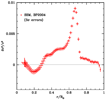 Fig
1: The difference in the squared sound speed between the Sun and a
standard solar model. The differences were obtained by inverting the
difference between oscillation frequencies of the Sun and those of the
model. The solar oscillation frequencies were obtained my the Michelson
Doppler Imager (MDI; see link in box to the right). Note that the
sound-speed profile of the model agrees to within fractions of a
percent with the sound-speed profile of the Sun. The small
difference in the core gives us an indication that the solar neutrino
problem cannot be a result of a deficient solar model (if the
model were bad, the differences between the Sun and the model would be
much larger). In fact, non-standard models constructed with an
aim to solve the neutrino problem have much larger differences
with respect to the Sun. Observations made by the Sudbury Neutrino
Observatory confirm that the solution of the solar neutrino problem
lies not with the standard solar model, but with the standard model of
particle physics that assumes that neutrinos are massless particles.
Fig
1: The difference in the squared sound speed between the Sun and a
standard solar model. The differences were obtained by inverting the
difference between oscillation frequencies of the Sun and those of the
model. The solar oscillation frequencies were obtained my the Michelson
Doppler Imager (MDI; see link in box to the right). Note that the
sound-speed profile of the model agrees to within fractions of a
percent with the sound-speed profile of the Sun. The small
difference in the core gives us an indication that the solar neutrino
problem cannot be a result of a deficient solar model (if the
model were bad, the differences between the Sun and the model would be
much larger). In fact, non-standard models constructed with an
aim to solve the neutrino problem have much larger differences
with respect to the Sun. Observations made by the Sudbury Neutrino
Observatory confirm that the solution of the solar neutrino problem
lies not with the standard solar model, but with the standard model of
particle physics that assumes that neutrinos are massless particles.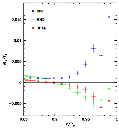 Fig. 2: The relative difference in the adiabatic index Gamma1
between the Sun and solar models constructed with different equations
of state. Only the "intrinsic" difference, i.e., the difference
independent of the differences in structure and helium abundance, is
shown. Note that the old EFF equation of state fairs very badly, but
the more modern MHD and OPAL equations of state are deficient too. As
in Fig. 1, these differences were obtained by inverting frequency
differences between the Sun and the models.
Fig. 2: The relative difference in the adiabatic index Gamma1
between the Sun and solar models constructed with different equations
of state. Only the "intrinsic" difference, i.e., the difference
independent of the differences in structure and helium abundance, is
shown. Note that the old EFF equation of state fairs very badly, but
the more modern MHD and OPAL equations of state are deficient too. As
in Fig. 1, these differences were obtained by inverting frequency
differences between the Sun and the models.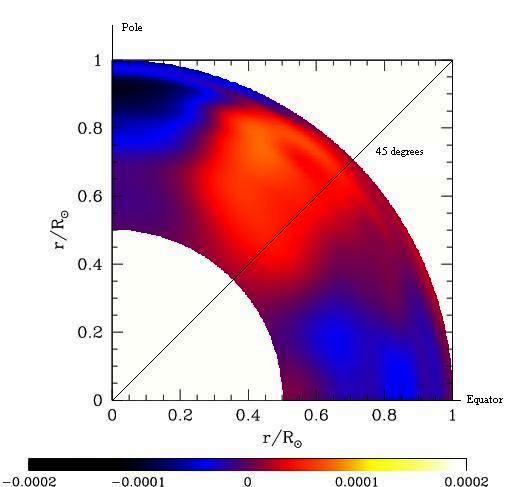 Fig.
3: The latitudinal distribution of solar sound speed plotted as a
function of latitude and radius.. The quantity plotted is actually the
relative departure from the spherically symmetric sound speed shown in
Fig. 1 above. Note that the asphericity of the solar sound-speed
distribution is small. The figure shows that the solar equatorial
regions are cooler than the mid-latitude regions.
Fig.
3: The latitudinal distribution of solar sound speed plotted as a
function of latitude and radius.. The quantity plotted is actually the
relative departure from the spherically symmetric sound speed shown in
Fig. 1 above. Note that the asphericity of the solar sound-speed
distribution is small. The figure shows that the solar equatorial
regions are cooler than the mid-latitude regions. Fig.
4: The solar rotation rate as a function of radius and latitude. These
results were obtained by inverting frequency splittings obtained by the
Global Oscillation Network Group (GONG). The rotation rate is given in
nHz. The equator rotates with a period of roughly 25 days and the pole
around 32 days. The dotted line 0.713R marks the position of the
base of the convection zone. The of the steep change in rotation rate
near the position of the base of the convection zone is usually
referred to as the "tachocline" and is believed to be the seat of the
solar dynamo. Also seen is a shear layer close to the solar surface,
and it can be seen that the maximum value of the solar rotation is
around a radius of 0.95R at the solar equator.
Fig.
4: The solar rotation rate as a function of radius and latitude. These
results were obtained by inverting frequency splittings obtained by the
Global Oscillation Network Group (GONG). The rotation rate is given in
nHz. The equator rotates with a period of roughly 25 days and the pole
around 32 days. The dotted line 0.713R marks the position of the
base of the convection zone. The of the steep change in rotation rate
near the position of the base of the convection zone is usually
referred to as the "tachocline" and is believed to be the seat of the
solar dynamo. Also seen is a shear layer close to the solar surface,
and it can be seen that the maximum value of the solar rotation is
around a radius of 0.95R at the solar equator. SOLAR ABUNDANCES:
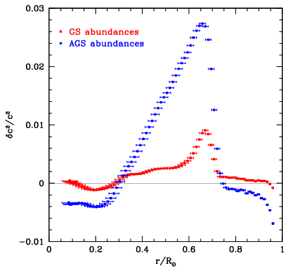
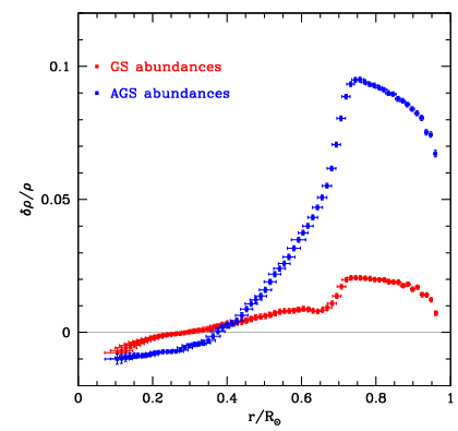 Fig
5: There is an ongoing controversy about Z/X, the solar heavy
metal abundance. Till about 2004, Z/X of the Sun was
believed to be 0.023, as was found by Grevesse & Sauval (1998).
However, since 2004, a new type of analysis indicated that solar
Z/X is much lower, and is about 0.0165 (Asplund, Grevesse &
Sauval 2005). Solar models constructed with the lower abundance,
however, show much larger differences with respect to the Sun
compared with models constructed with the older, higher abundances.
This can be seen from these figures. The panel on the left shows the
relative sound speed difference between a model constructed with
the higher abundances (shown in red) and with a model constructed
with the lower abundances (blue). The panel on the right shows the
relative density differences between the Sun and the two models. Note
that the differences are much smaller for the high-abundance model.
This and other helioseismic results indicate that the solar Z/X
is high and that the analysis that resulted in the low abundances
suffer from some discrepancies. A review of the controversy can be
found in Basu & Antia (2008).
Fig
5: There is an ongoing controversy about Z/X, the solar heavy
metal abundance. Till about 2004, Z/X of the Sun was
believed to be 0.023, as was found by Grevesse & Sauval (1998).
However, since 2004, a new type of analysis indicated that solar
Z/X is much lower, and is about 0.0165 (Asplund, Grevesse &
Sauval 2005). Solar models constructed with the lower abundance,
however, show much larger differences with respect to the Sun
compared with models constructed with the older, higher abundances.
This can be seen from these figures. The panel on the left shows the
relative sound speed difference between a model constructed with
the higher abundances (shown in red) and with a model constructed
with the lower abundances (blue). The panel on the right shows the
relative density differences between the Sun and the two models. Note
that the differences are much smaller for the high-abundance model.
This and other helioseismic results indicate that the solar Z/X
is high and that the analysis that resulted in the low abundances
suffer from some discrepancies. A review of the controversy can be
found in Basu & Antia (2008).CHANGES IN SOLAR STRUCTURE AND DYNAMICS:
 Fig 6: The
solar rotation rate changes with change in the level of solar activity.
The change can be seen clearly by subtracting out the time averaged
rotation rate from the rotation rate at each epoch. This figure shows
the change in the rotation rate as a function of radius and
latitude.The results shown are in m/s and the error in the results is
of 1 m/s. These results were obtained with data obtained by GONG
over solar cycle 23. Note the shifting pattern of the changes.
Fig 6: The
solar rotation rate changes with change in the level of solar activity.
The change can be seen clearly by subtracting out the time averaged
rotation rate from the rotation rate at each epoch. This figure shows
the change in the rotation rate as a function of radius and
latitude.The results shown are in m/s and the error in the results is
of 1 m/s. These results were obtained with data obtained by GONG
over solar cycle 23. Note the shifting pattern of the changes.
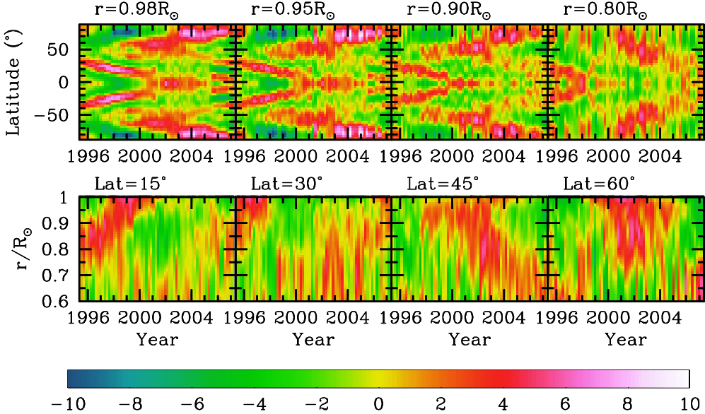 Fig
7: The same as in Fig. 6, except that we have plotted the changes in
rotation as a function of time and latitude for a few radii (top) and
as a function of time and radius at a few latitudes (bottom). The upper
panel shows a clear pattern of bands that migrate towards the equator
in the low-latitude regions, and the bands that move towards the poles
in the high-latitude region. This pattern is very similar to the
pattern of torsional oscillations observed at the solar surface, and
the flows are often referred to as zonal flows. The lower panel shows
that the zonal flow pattern moving upwards from near the base of the
convection zone as the solar cycle progresses. The pattern
migrates upwards with a speed of about 1 m/s.
Fig
7: The same as in Fig. 6, except that we have plotted the changes in
rotation as a function of time and latitude for a few radii (top) and
as a function of time and radius at a few latitudes (bottom). The upper
panel shows a clear pattern of bands that migrate towards the equator
in the low-latitude regions, and the bands that move towards the poles
in the high-latitude region. This pattern is very similar to the
pattern of torsional oscillations observed at the solar surface, and
the flows are often referred to as zonal flows. The lower panel shows
that the zonal flow pattern moving upwards from near the base of the
convection zone as the solar cycle progresses. The pattern
migrates upwards with a speed of about 1 m/s.
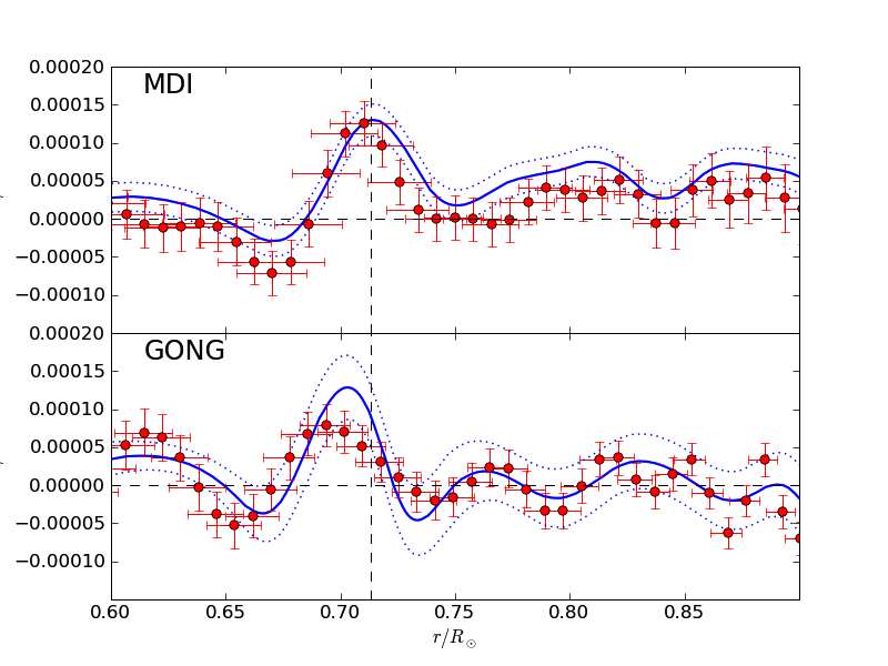 Fig.
8: Unlike the case of the solar rotation rate (Figs 6 and 7
above), change in solar structure in the deeper layers of the Sun
is small and have taken a long time to detect. The figure shows
the relative sound-speed difference between the Sun at the activity
maximum of cycle 23 and the Sun at the activity minimum prior to the
rise of cycle 23. Results obtained by both MDI and GONG data are shown,
the lines and the symbols show the results of two different types
of inversions. As can be seen, the differences are extremely small. The
difference at the base of the convection zone (marked by the vertical
line) corresponds to a change of magnetic field of about 300-400kG.
Special analysis techniques had to be used to obtain the result and
details can be found in Baldner & Basu (2008).
Fig.
8: Unlike the case of the solar rotation rate (Figs 6 and 7
above), change in solar structure in the deeper layers of the Sun
is small and have taken a long time to detect. The figure shows
the relative sound-speed difference between the Sun at the activity
maximum of cycle 23 and the Sun at the activity minimum prior to the
rise of cycle 23. Results obtained by both MDI and GONG data are shown,
the lines and the symbols show the results of two different types
of inversions. As can be seen, the differences are extremely small. The
difference at the base of the convection zone (marked by the vertical
line) corresponds to a change of magnetic field of about 300-400kG.
Special analysis techniques had to be used to obtain the result and
details can be found in Baldner & Basu (2008).
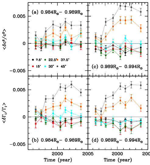 Fig.
9: While changes in structure in the deeper layers of the Sun are small
(and difficult to detect), changes in the near-surface layers are
larger and somewhat easier to detect. Changes in the latitudinal
distribution of solar sound-speed are particularly large. The figure
shows the relative difference in sound-speed and the relative
difference in the adiabatic index between the equator and a few
latitudes as a function of time. Results averaged over two radius
ranges are shown. We can see that not only does the sound-speed and
adiabatic index change with time, different latitudes show a different
magnitude of change.
Fig.
9: While changes in structure in the deeper layers of the Sun are small
(and difficult to detect), changes in the near-surface layers are
larger and somewhat easier to detect. Changes in the latitudinal
distribution of solar sound-speed are particularly large. The figure
shows the relative difference in sound-speed and the relative
difference in the adiabatic index between the equator and a few
latitudes as a function of time. Results averaged over two radius
ranges are shown. We can see that not only does the sound-speed and
adiabatic index change with time, different latitudes show a different
magnitude of change.
ACTIVE REGIONS:
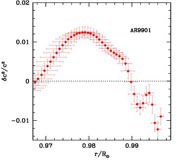 Fig.
8: Helioseismic techniques can be used to study the thermal
structure of active regions. The figure shows the relative sound-speed
difference between active region AR9901 and an adjacent quiet region.
It can be seen that the sound speed of the active region is lower than
that of the quiet region till a depth of about 7Mm, and then the
sound-speed of the active region becomes larger. The magnitude of the
difference (both the negative region close to the surface and the
positive region deeper) depends on the magnetic field strength of the
active region.
Fig.
8: Helioseismic techniques can be used to study the thermal
structure of active regions. The figure shows the relative sound-speed
difference between active region AR9901 and an adjacent quiet region.
It can be seen that the sound speed of the active region is lower than
that of the quiet region till a depth of about 7Mm, and then the
sound-speed of the active region becomes larger. The magnitude of the
difference (both the negative region close to the surface and the
positive region deeper) depends on the magnetic field strength of the
active region.
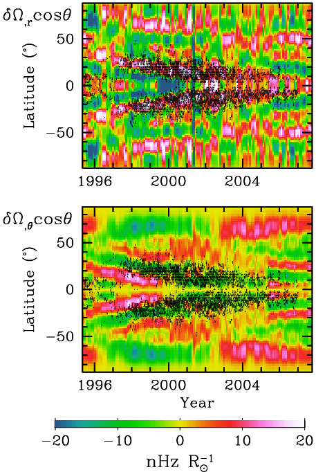 Fig. 9: There appears to be a close correlation between changes
in the solar rotation rate and the positions where sunspots emerge. In
particular, the correlation is between changes in the radial and
latitudinal gradients of the
solar rotation rate and the positions of sunspot emerge. This is shown
in the figure. The colour image shows the change in the radial gradient
as a function of time and latitude (top) and the change in the
latitudinal gradient as a function of time and latitude (bottom) at
0.98R. The points mark the position of sunspots. Sunspots appear to
concentrate in low-latitude regions where the variation in the radial
gradient is positive but the variation of the latitudinal gradient is
negative.
Fig. 9: There appears to be a close correlation between changes
in the solar rotation rate and the positions where sunspots emerge. In
particular, the correlation is between changes in the radial and
latitudinal gradients of the
solar rotation rate and the positions of sunspot emerge. This is shown
in the figure. The colour image shows the change in the radial gradient
as a function of time and latitude (top) and the change in the
latitudinal gradient as a function of time and latitude (bottom) at
0.98R. The points mark the position of sunspots. Sunspots appear to
concentrate in low-latitude regions where the variation in the radial
gradient is positive but the variation of the latitudinal gradient is
negative.
Fig 6: The
solar rotation rate changes with change in the level of solar activity.
The change can be seen clearly by subtracting out the time averaged
rotation rate from the rotation rate at each epoch. This figure shows
the change in the rotation rate as a function of radius and
latitude.The results shown are in m/s and the error in the results is
of 1 m/s. These results were obtained with data obtained by GONG
over solar cycle 23. Note the shifting pattern of the changes. Fig
7: The same as in Fig. 6, except that we have plotted the changes in
rotation as a function of time and latitude for a few radii (top) and
as a function of time and radius at a few latitudes (bottom). The upper
panel shows a clear pattern of bands that migrate towards the equator
in the low-latitude regions, and the bands that move towards the poles
in the high-latitude region. This pattern is very similar to the
pattern of torsional oscillations observed at the solar surface, and
the flows are often referred to as zonal flows. The lower panel shows
that the zonal flow pattern moving upwards from near the base of the
convection zone as the solar cycle progresses. The pattern
migrates upwards with a speed of about 1 m/s. Fig.
8: Unlike the case of the solar rotation rate (Figs 6 and 7
above), change in solar structure in the deeper layers of the Sun
is small and have taken a long time to detect. The figure shows
the relative sound-speed difference between the Sun at the activity
maximum of cycle 23 and the Sun at the activity minimum prior to the
rise of cycle 23. Results obtained by both MDI and GONG data are shown,
the lines and the symbols show the results of two different types
of inversions. As can be seen, the differences are extremely small. The
difference at the base of the convection zone (marked by the vertical
line) corresponds to a change of magnetic field of about 300-400kG.
Special analysis techniques had to be used to obtain the result and
details can be found in Baldner & Basu (2008). Fig.
9: While changes in structure in the deeper layers of the Sun are small
(and difficult to detect), changes in the near-surface layers are
larger and somewhat easier to detect. Changes in the latitudinal
distribution of solar sound-speed are particularly large. The figure
shows the relative difference in sound-speed and the relative
difference in the adiabatic index between the equator and a few
latitudes as a function of time. Results averaged over two radius
ranges are shown. We can see that not only does the sound-speed and
adiabatic index change with time, different latitudes show a different
magnitude of change. ACTIVE REGIONS:
Fig.
8: Helioseismic techniques can be used to study the thermal
structure of active regions. The figure shows the relative sound-speed
difference between active region AR9901 and an adjacent quiet region.
It can be seen that the sound speed of the active region is lower than
that of the quiet region till a depth of about 7Mm, and then the
sound-speed of the active region becomes larger. The magnitude of the
difference (both the negative region close to the surface and the
positive region deeper) depends on the magnetic field strength of the
active region.
Fig. 9: There appears to be a close correlation between changes
in the solar rotation rate and the positions where sunspots emerge. In
particular, the correlation is between changes in the radial and
latitudinal gradients of the
solar rotation rate and the positions of sunspot emerge. This is shown
in the figure. The colour image shows the change in the radial gradient
as a function of time and latitude (top) and the change in the
latitudinal gradient as a function of time and latitude (bottom) at
0.98R. The points mark the position of sunspots. Sunspots appear to
concentrate in low-latitude regions where the variation in the radial
gradient is positive but the variation of the latitudinal gradient is
negative.